What makes a red wine score well?

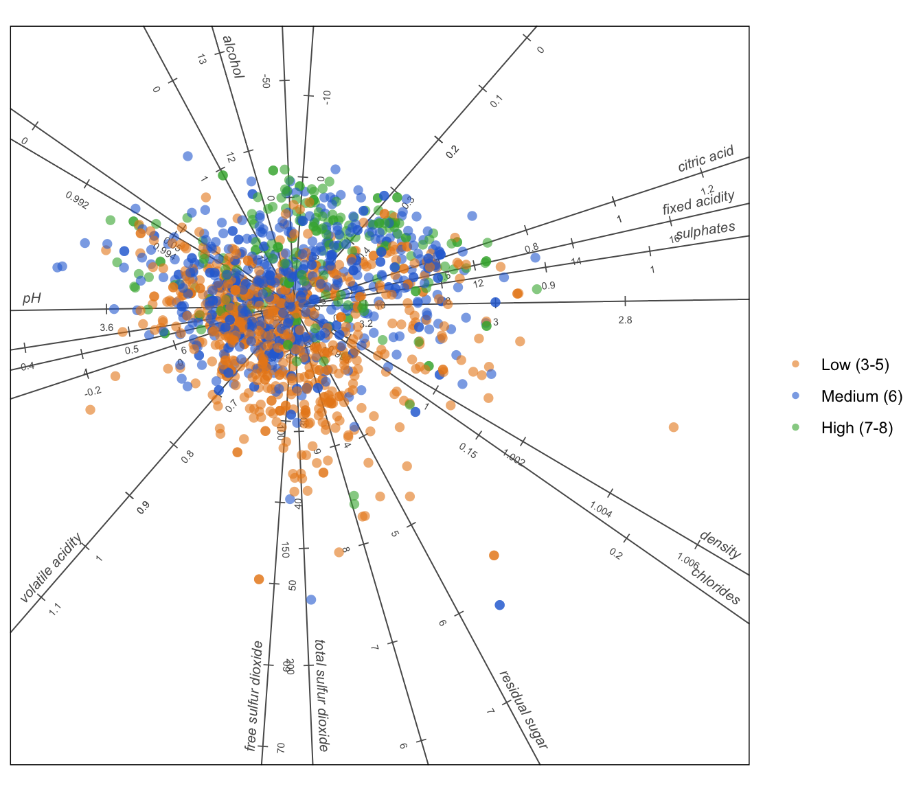
A PCA biplot of 1 599 Portuguese red wines shows which chemical properties travel together and which ones separate the high-scoring wines from the rest.

The data

The wine quality data set was collected by Cortez and colleagues in 2009. It records eleven physicochemical measurements for 1 599 red vinho verde wines from the north of Portugal, such as acidity, sugar, alcohol and sulphur dioxide, together with a quality score from 0 to 10 awarded by a panel of tasters.

Each row is one wine. The eleven measurements are the variables we will draw as axes. The quality score is used only to colour the points, so we can see whether chemistry and taste agree.

The question

Wine chemistry is measured in a lab. Wine quality is judged by people. Do the wines that people like share a chemical profile, and if so, which measurements matter?

The biplot

# Development version of biplotEZ, installed from GitHub with
#   remotes::install_github("MuViSU/biplotEZ")
# It draws with ggplot2, so install.packages("ggplot2") if needed.
library(biplotEZ)

wine <- read.csv("winequality-red.csv", sep = ";")

# Group wines into three quality bands so the colouring is easy to read
wine$band <- cut(wine$quality,
                 breaks = c(0, 5, 6, 10),
                 labels = c("Low (3-5)", "Medium (6)", "High (7-8)"))

# Tidy the variable names for the plot
names(wine) <- gsub("\\.", " ", names(wine))

biplot(wine[, 1:11], group.aes = wine$band, scaled = TRUE) |>
  PCA() |>
  samples(col = c("#E8891C", "#2A6FD6", "#3FAF3A"), pch = 16, opacity = 0.6) |>
  axes(col = "grey35", label.cex = 0.75) |>
  plot()

PCA biplot of 1 599 red wines. Points are wines, coloured by quality band. Each labelled axis is one chemical measurement; a wine’s projection onto an axis approximates its value for that measurement.

What the picture tells us

Because the eleven measurements are on very different scales (alcohol in percent, sulphur dioxide in milligrams per litre), each variable was standardised before the biplot was built. The plot then shows the two directions in which the wines vary most.

Axes that point the same way measure the same thing. Fixed acidity and citric acid run almost parallel, and pH points the opposite way. That is the chemistry being explained: more acid means lower pH. Density and chlorides also travel together, pointing away from alcohol, because alcohol is lighter than water. Similarly, free and total sulphur dioxide point together because one is a component of the other.

High-scoring wines sit on one side. The green points drift towards the alcohol axis and away from the volatile acidity axis. Volatile acidity is essentially vinegar, so wines with more of it score lower, while wines with more alcohol and more sulphates tend to score higher. The low-scoring orange points lean the other way.

Chemistry only partly explains taste. The bands overlap heavily. Chemistry pushes a wine in a direction, but the tasting panel clearly responds to things the lab does not measure.

Take-aways

• Alcohol and sulphates are associated with higher scores; volatile acidity with lower scores.
• Several measurements are near duplicates of each other, so the eleven variables carry far fewer than eleven separate pieces of information.
• A biplot puts all of this in one picture: the groupings of wines, the relationships between measurements, and the link between the two.

NoteReproduce this post

This post uses the development version of biplotEZ from GitHub. Install it with remotes::install_github("MuViSU/biplotEZ"), then run the code chunks above. The data file winequality-red.csv sits next to this post and was downloaded from the UCI Machine Learning Repository.