moveEZ

Overview

moveEZ extends the biplotEZ package (Lubbe et al. 2024) to animate PCA biplots across the ordered levels of a categorical variable, referred to throughout as the time variable. Rather than producing a separate static biplot per level — which fragments sequential information and makes gradual structural change difficult to perceive — moveEZ renders transitions between levels as a continuous animation.

The package provides three animation functions of increasing methodological complexity:

moveplot(): animates sample positions against fixed variable vectors, computed once on the full dataset.
moveplot2(): animates both sample positions and variable vectors, computed separately per time slice, with optional manual alignment.
moveplot3(): extends moveplot2() with automated alignment via Generalised Procrustes Analysis (GPA) (Gower and Dijksterhuis 2004).

All three functions support both animated output (move = TRUE) and static faceted output (move = FALSE), the latter being useful for publication figures or detailed inspection of individual time slices.

For a full methodological treatment, including the theoretical motivation for each framework and a discussion of sign indeterminacy in sequential PCA, refer to the accompanying paper.

Data

Throughout this vignette we use the Africa_climate dataset included in moveEZ. This dataset contains climate measurements for ten African regions derived from the ERA5 reanalysis (Hersbach et al. 2023), with IPCC-defined reference regions (Iturbide et al. 2020) as the grouping variable. Measurements span from 1950 to 2020 in ten-year increments, with twelve monthly observations per region per year. The six continuous variables are described below:

Variable	Unit	Description
Accumulated Precipitation (AP)	m/day	Total daily precipitation
Daily Evaporation (DE)	m/day	Net daily evaporation
Temperature (Temp)	°C	Mean daily surface temperature
Soil Moisture (SM)	m³/m³	Volumetric water content of upper soil layer
Standardised Precipitation Index (SPI6)	Dimensionless	6-month precipitation anomaly index
Wind Speed (Wind)	m/s	Mean daily wind speed at 10m

data("Africa_climate")
tibble::tibble(Africa_climate)
#> # A tibble: 960 × 9
#>    Year  Month     Region AccPrec DailyEva  Temp SoilMois  SPI6  wind
#>    <fct> <fct>     <fct>    <dbl>    <dbl> <dbl>    <dbl> <dbl> <dbl>
#>  1 1950  January   ARP      0.177  0.0316   14.8    2.75  1.62   4.07
#>  2 1950  February  ARP      0.208 -0.0249   15.4    2.22  1.32   4.24
#>  3 1950  March     ARP      0.306  0.0122   20.9    2.08  0.987  4.04
#>  4 1950  April     ARP      0.196  0.00396  24.8    1.73  0.916  3.72
#>  5 1950  May       ARP      0.590 -0.0448   28.4    2.47  0.691  3.91
#>  6 1950  June      ARP      0.32  -0.00754  30.4    1.17  0.249  4.40
#>  7 1950  July      ARP      1.33   0.00184  30.8    2.00  0.673  4.93
#>  8 1950  August    ARP      1.82  -0.00944  30.5    2.67  0.937  4.45
#>  9 1950  September ARP      0.706 -0.0107   29.7    1.98  1.22   3.67
#> 10 1950  October   ARP      0.102 -0.0259   25.9    0.976 1.65   3.18
#> # ℹ 950 more rows

All examples in this vignette use a PCA biplot constructed on the full Africa_climate dataset as the base object, passed to each moveplot function via the pipe operator:

bp <- biplot(Africa_climate, scaled = TRUE) |>
  PCA(group.aes = Africa_climate$Region) |>
  samples(opacity = 0.8, col = scales::hue_pal()(10)) |>
  plot()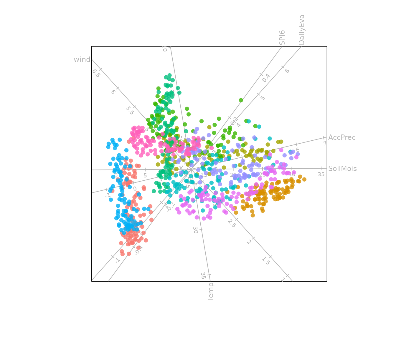

Fixed Variable Frame: `moveplot()`

moveplot() computes a single PCA decomposition on the full dataset. The variable vectors remain fixed throughout the animation, providing a stable reference frame. Only the sample positions — sliced according to the levels of the time variable — are animated sequentially. This approach is most appropriate when the underlying variance–covariance structure can be assumed stable across time, and is the only viable option when there is a single observation per group per time level.

The key arguments are:

time.var: the name of the ordered categorical variable defining the sequential structure (e.g. "Year").
group.var: the name of the grouping variable, used for colour-coding (e.g. "Region").
hulls: logical; when TRUE convex hulls summarise group spread at each time level; when FALSE individual sample points are displayed. Hulls require at least three observations per group per time level — if fewer exist, points are plotted automatically.
move: logical; TRUE produces an animation, FALSE produces a static faceted display.
shadow: logical; available only when hulls = FALSE. When TRUE, faded traces of previous sample positions are retained in the animation, conveying the direction and speed of movement across time.
scale.var: numeric multiplier applied to variable vectors to improve visibility.

Static faceted display

bp |> moveplot(time.var = "Year", group.var = "Region",
               hulls = TRUE, move = FALSE)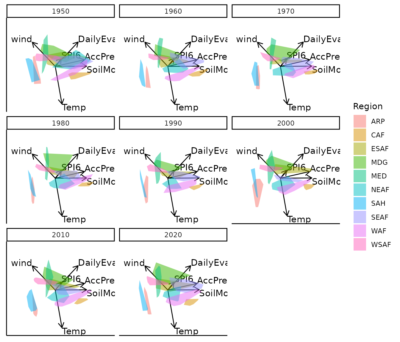

#> Object of class biplot, based on 960 samples and 9 variables.
#> 6 numeric variables.
#> 3 categorical variables.

Animated display

The animation reveals how the regional climate configurations shift relative to the fixed variable vectors across decades. Regions that move in the direction of a variable vector are increasing on that variable over time; regions moving against the vector are decreasing.

Dynamic Frame: `moveplot2()`

moveplot2() computes a separate PCA decomposition for each time slice, allowing both sample positions and variable vectors to evolve across levels. This provides a more faithful depiction of time-varying variance–covariance structures but introduces a practical complication: eigenvectors are determined only up to a sign change, meaning that consecutive time slices may produce biplots that are reflections of one another. This sign indeterminacy is mathematically inconsequential but visually disruptive.

Two additional arguments address this:

align.time: a vector of time levels at which alignment should be applied.
reflect: specifies the axis of reflection — "x", "y", or "xy" — with each entry corresponding to a level in align.time. Both arguments accept vectors when alignment is needed at multiple time levels.

Static faceted display (unaligned)

bp |> moveplot2(time.var = "Year", group.var = "Region",
                hulls = TRUE, move = FALSE)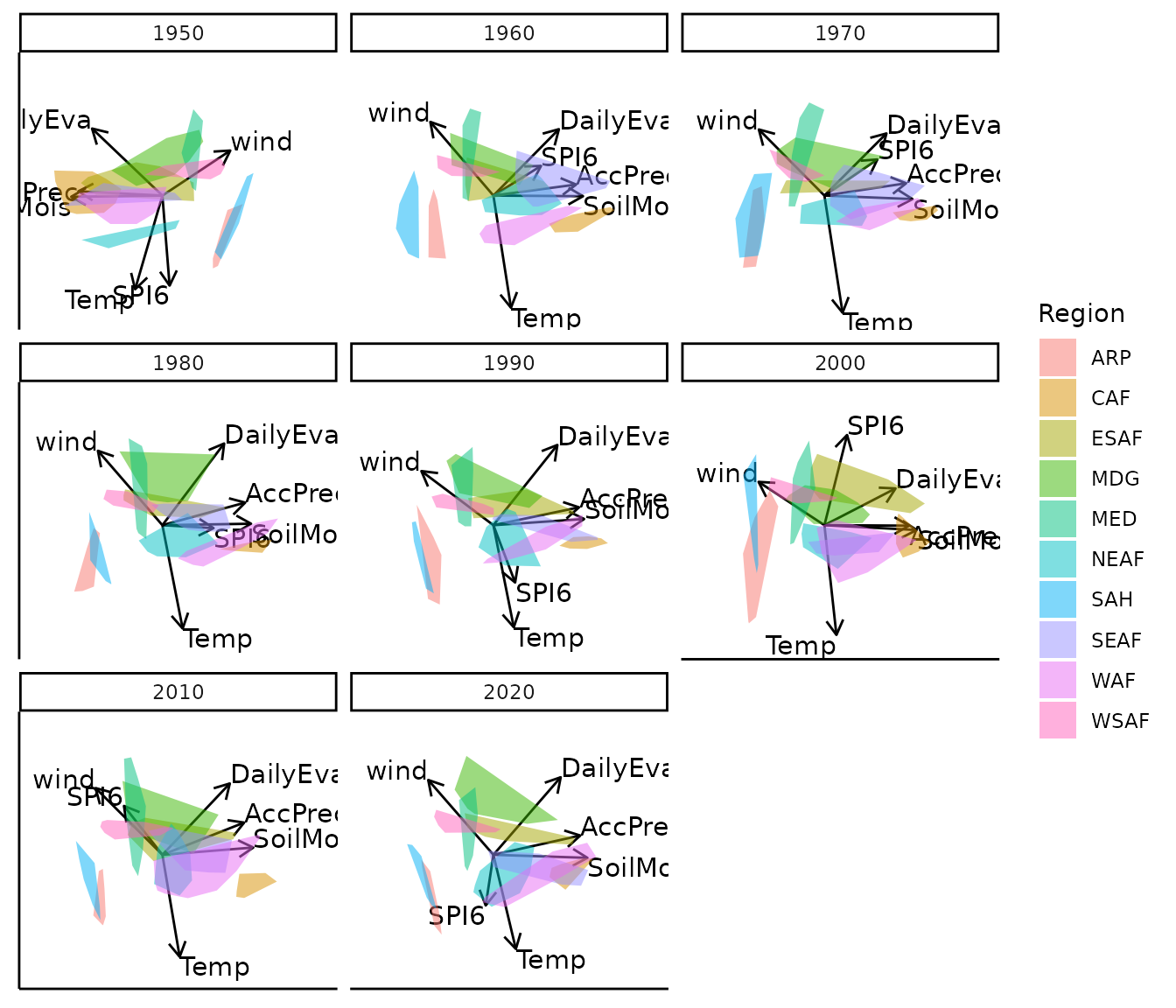

#> Object of class biplot, based on 960 samples and 9 variables.
#> 6 numeric variables.
#> 3 categorical variables.

Note the discontinuity between 1950 and 1960 — the variable vectors and sample configuration are reflected about the x-axis. This is a sign indeterminacy artefact, not a genuine structural change.

Static faceted display (aligned)

bp |> moveplot2(time.var = "Year", group.var = "Region",
                hulls = TRUE, move = FALSE,
                align.time = "1950", reflect = "x")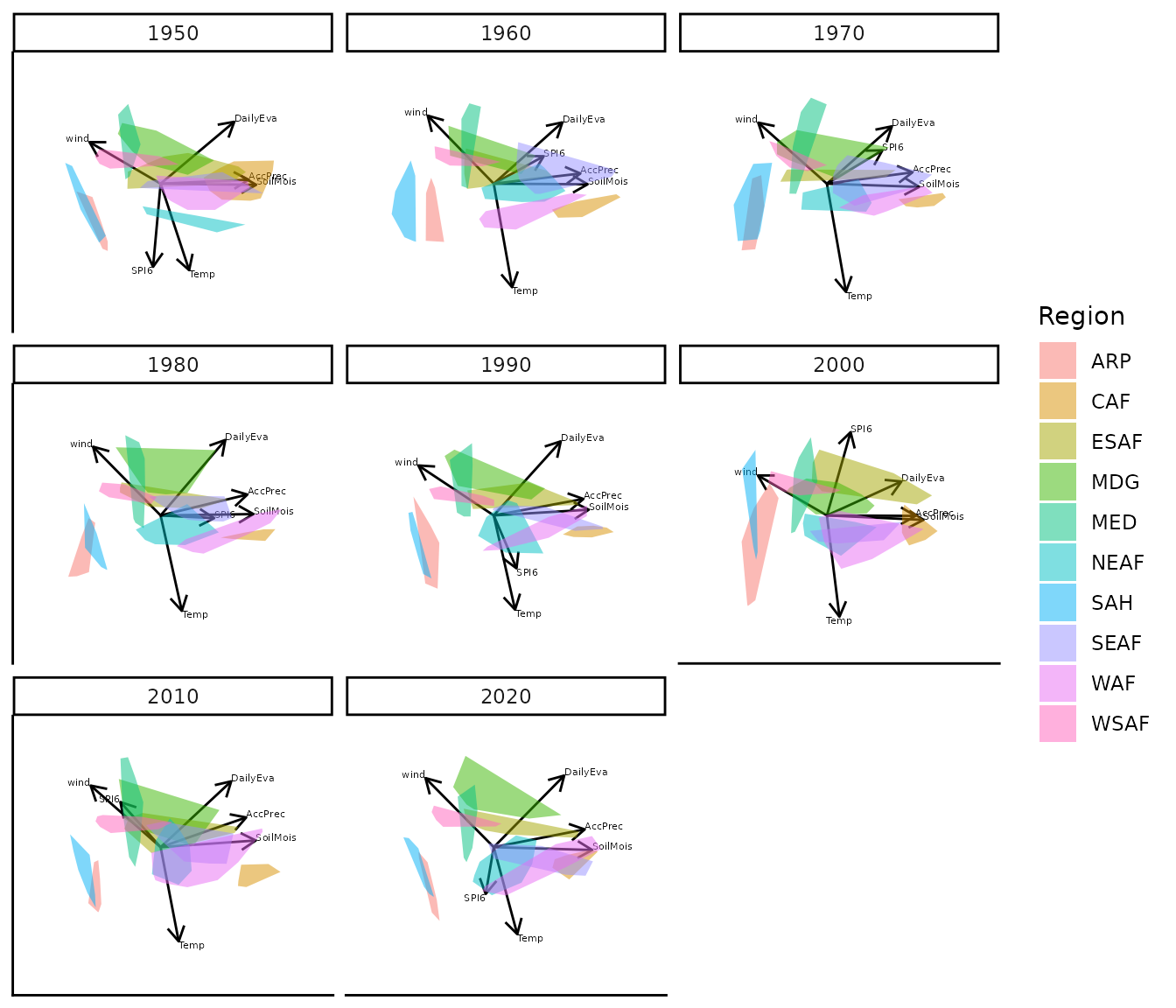

#> Object of class biplot, based on 960 samples and 9 variables.
#> 6 numeric variables.
#> 3 categorical variables.

Applying a reflection about the x-axis at 1950 restores visual continuity across the sequence of biplots.

Animated display

Automated Alignment: `moveplot3()`

moveplot3() automates the alignment of sequential biplots using GPA (Gower and Dijksterhuis 2004), implemented via the GPAbin package (Nienkemper-Swanepoel et al. 2023). GPA iteratively applies admissible transformations — translation, reflection, rotation, and scaling — to minimise the sum of squared distances between each time slice and a target configuration, without requiring the user to manually identify discontinuities.

The target argument controls what the time slices are aligned to:

target = NULL: aligns all time slices to their average (consensus) configuration.
target = <dataset>: aligns all time slices to a user-supplied reference dataset containing measurements on the same variables.

The Africa_climate_target dataset included in moveEZ provides 1989 measurements on the same variables as Africa_climate, and is used here as an external reference.

Consensus target (`target = NULL`)

Static faceted display

bp |> moveplot3(time.var = "Year", group.var = "Region",
                hulls = TRUE, move = FALSE, target = NULL)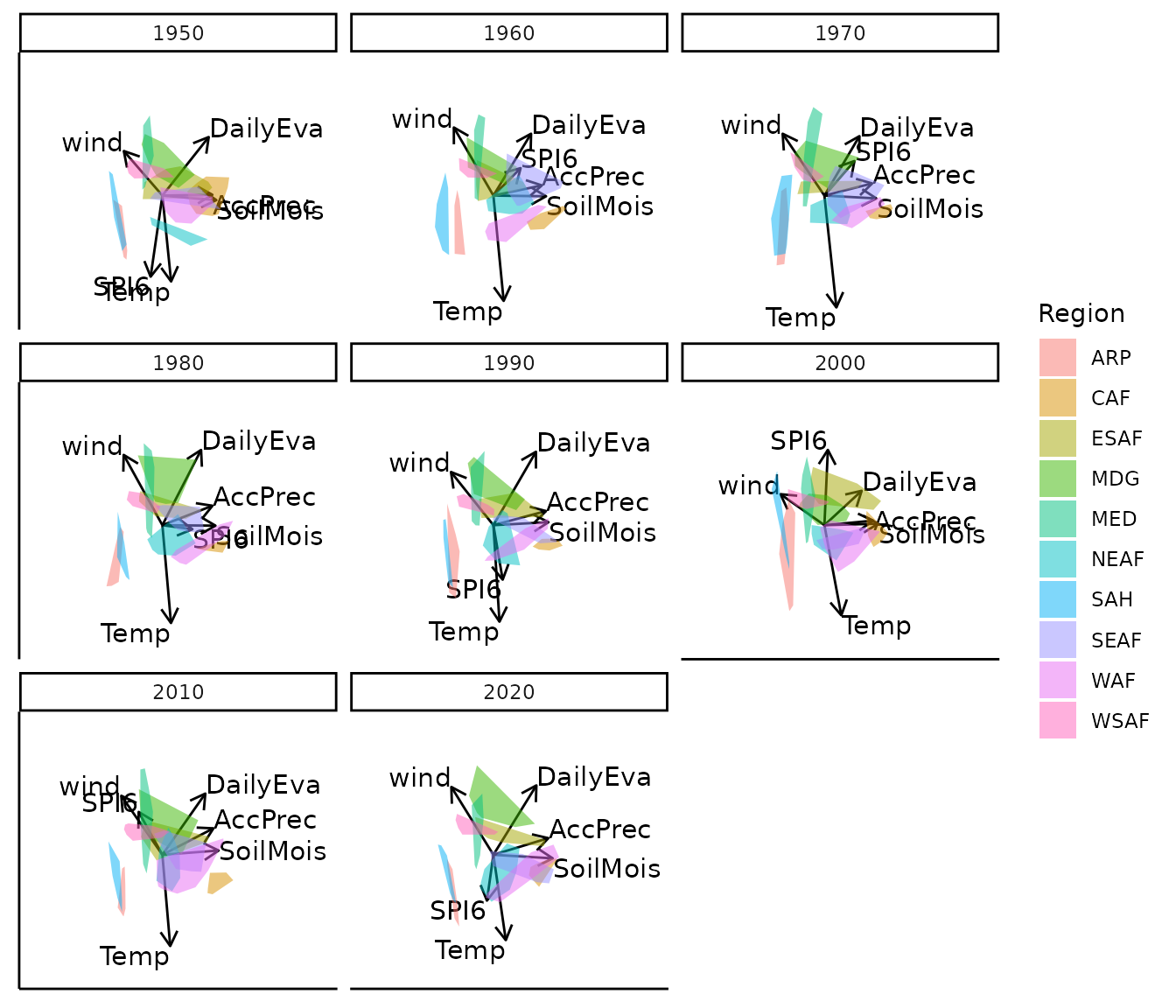

#> Object of class biplot, based on 960 samples and 9 variables.
#> 6 numeric variables.
#> 3 categorical variables.

All time slices are aligned to the average configuration across years, producing a consistently oriented sequence of biplots without manual intervention.

Animated display

User-supplied target (`target = Africa_climate_target`)

data("Africa_climate_target")
tibble::tibble(Africa_climate_target)
#> # A tibble: 120 × 9
#>    Year  Month     Region AccPrec DailyEva  Temp SoilMois     SPI6  wind
#>    <fct> <chr>     <chr>    <dbl>    <dbl> <dbl>    <dbl>    <dbl> <dbl>
#>  1 1989  January   ARP     0.0740 -0.00416  14.9    1.11  -1.08     4.06
#>  2 1989  February  ARP     0.235  -0.00161  17.3    1.55  -0.817    4.19
#>  3 1989  March     ARP     0.815  -0.0220   21.5    2.70   0.00329  4.12
#>  4 1989  April     ARP     0.495   0.0508   25.0    2.90   0.226    3.48
#>  5 1989  May       ARP     0.0411 -0.0130   30.1    1.08   0.306    3.96
#>  6 1989  June      ARP     0.0693 -0.0234   31.6    0.633  0.261    4.33
#>  7 1989  July      ARP     0.0833 -0.0164   33.1    0.606  0.527    4.36
#>  8 1989  August    ARP     0.137  -0.0209   32.6    0.685  0.575    4.05
#>  9 1989  September ARP     0.102  -0.0246   30.1    0.656  0.0360   3.56
#> 10 1989  October   ARP     0.0330 -0.0549   26.5    0.449 -0.919    3.45
#> # ℹ 110 more rows

Static faceted display

bp |> moveplot3(time.var = "Year", group.var = "Region",
                hulls = TRUE, move = FALSE,
                target = Africa_climate_target)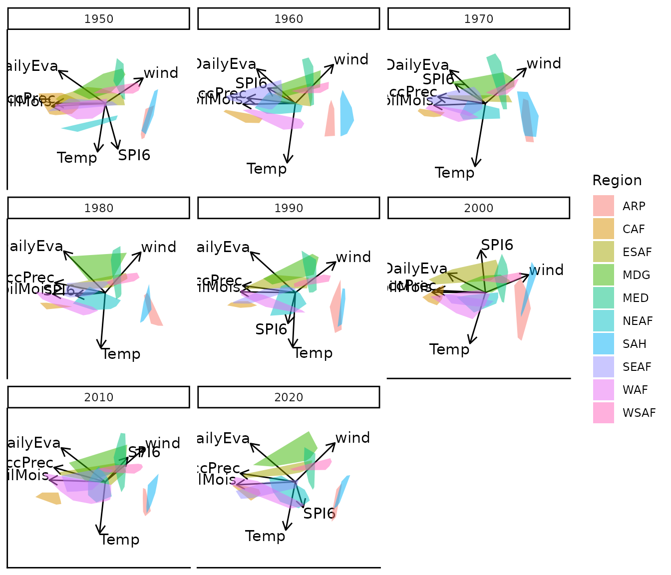

#> Object of class biplot, based on 960 samples and 9 variables.
#> 6 numeric variables.
#> 3 categorical variables.

Each time slice is aligned to the 1989 reference configuration, exposing the structural differences between 1989 and each decade from 1950 to 2020. Note that the target biplot itself is not shown in this display — it serves only as the alignment reference. To visualise the target configuration separately, pass it to moveplot() directly:

viz_1989 <- Africa_climate_target |>
  dplyr::mutate(
    Target = as.factor(rep("1989", nrow(Africa_climate_target))),
    Region = as.factor(Region)
  )

bp_1989 <- biplot(viz_1989, scaled = TRUE) |>
  PCA(group.aes = viz_1989$Region)

bp_1989 |> moveplot(time.var = "Target", group.var = "Region",
                    hulls = TRUE, move = FALSE)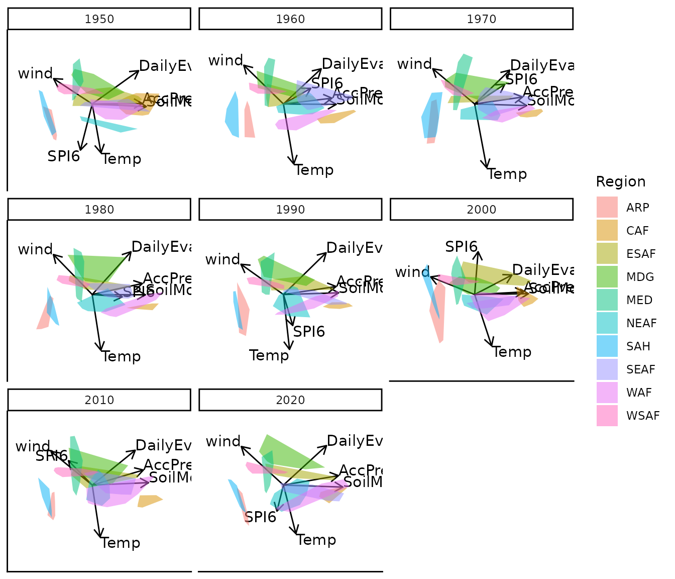

#> Object of class biplot, based on 120 samples and 10 variables.
#> 6 numeric variables.
#> 4 categorical variables.

Animated display

Evaluation

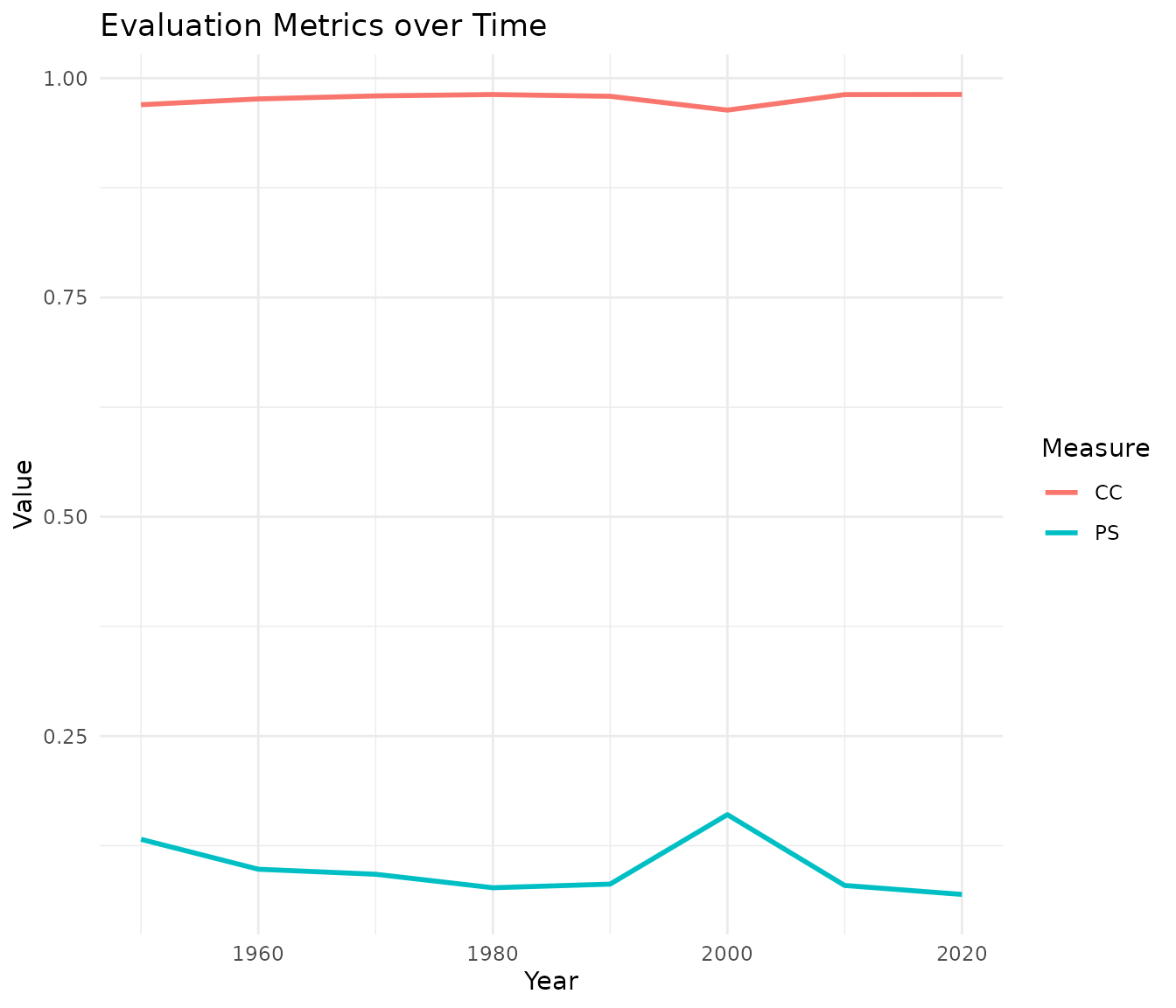
The evaluation() function quantifies the magnitude of structural change between each time slice and the target configuration specified in moveplot3(). It provides five measures based on orthogonal Procrustes analysis, in two categories:

Fit measures (values closer to their optimal indicate better similarity):

PS (Procrustes Statistic): optimal value is 0.
CC (Congruence Coefficient): optimal value is 1.

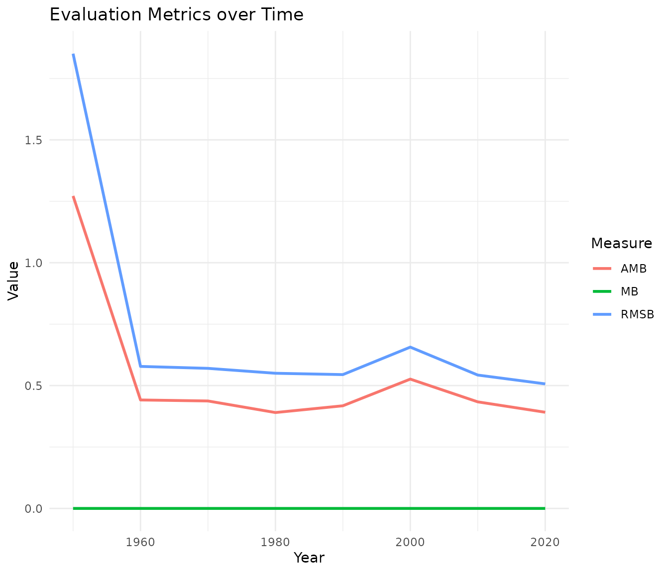
Bias measures (lower values indicate less systematic distortion):

AMB (Absolute Mean Bias)
MB (Mean Bias): a value near zero indicates no systematic directional shift.
RMSB (Root Mean Squared Bias)

results <- bp |>
  moveplot3(time.var = "Year", group.var = "Region",
            hulls = TRUE, move = FALSE, target = NULL) |>
  evaluation()

Numerical measures

results$eval.list
#> [[1]]
#>      Target vs. 1950
#> PS            0.1323
#> CC            0.9697
#> AMB           1.2717
#> MB            0.0000
#> RMSB          1.8506
#> 
#> [[2]]
#>      Target vs. 1960
#> PS            0.0982
#> CC            0.9763
#> AMB           0.4414
#> MB            0.0000
#> RMSB          0.5779
#> 
#> [[3]]
#>      Target vs. 1970
#> PS            0.0925
#> CC            0.9798
#> AMB           0.4373
#> MB            0.0000
#> RMSB          0.5701
#> 
#> [[4]]
#>      Target vs. 1980
#> PS            0.0771
#> CC            0.9813
#> AMB           0.3903
#> MB            0.0000
#> RMSB          0.5501
#> 
#> [[5]]
#>      Target vs. 1990
#> PS            0.0812
#> CC            0.9793
#> AMB           0.4177
#> MB            0.0000
#> RMSB          0.5446
#> 
#> [[6]]
#>      Target vs. 2000
#> PS            0.1604
#> CC            0.9636
#> AMB           0.5263
#> MB            0.0000
#> RMSB          0.6564
#> 
#> [[7]]
#>      Target vs. 2010
#> PS            0.0797
#> CC            0.9813
#> AMB           0.4337
#> MB            0.0000
#> RMSB          0.5428
#> 
#> [[8]]
#>      Target vs. 2020
#> PS            0.0695
#> CC            0.9814
#> AMB           0.3914
#> MB            0.0000
#> RMSB          0.5069

Fit measures over time

results$fit.plot

The biplot for 2000 shows a notably lower CC and higher PS relative to other years, indicating a structural departure from the consensus configuration that warrants closer investigation.

Bias measures over time

results$bias.plot

The initial bias at 1950 is high but decreases and stabilises from 1960, with an increase in AMB and RMSB at 2000 consistent with the fit measures. The MB remains close to zero throughout, confirming no systematic directional bias in the alignment.

Additional Examples

Alternative use of `time.var`

The group variable can be specified as the time variable to produce a faceted display in which each panel shows a single group rather than a single time level. This can be useful when group-level patterns are difficult to distinguish in the standard faceted display, where all groups appear together in each panel.

bp |> moveplot(time.var = "Region", group.var = "Region",
               hulls = FALSE, move = FALSE)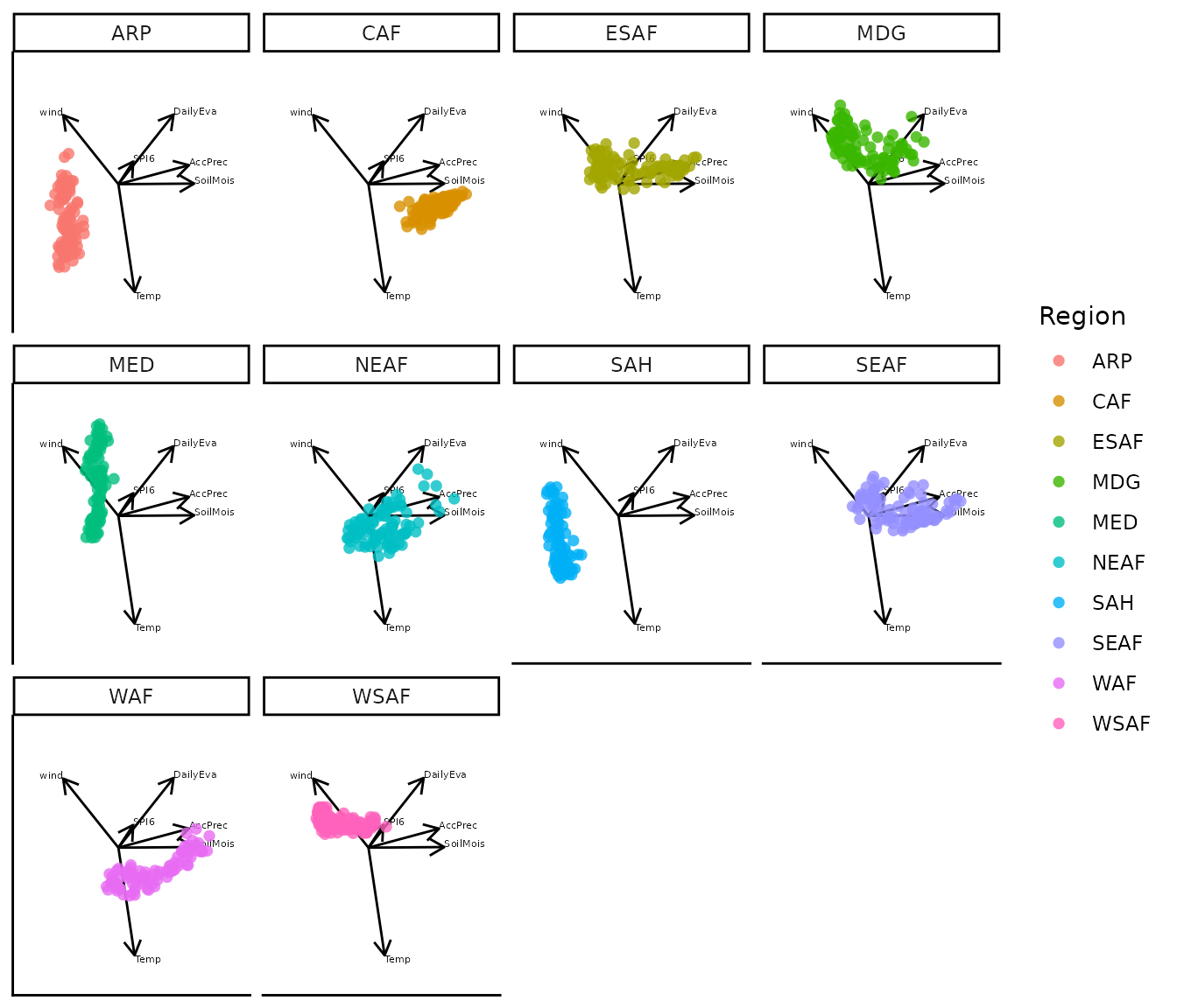

#> Object of class biplot, based on 960 samples and 9 variables.
#> 6 numeric variables.
#> 3 categorical variables.

Customising aesthetics

moveEZ inherits its core biplot construction from biplotEZ, and aesthetic customisation — such as point colours, plotting characters, and axis label sizes — should be specified in the biplotEZ biplot object before passing it to any moveplot function. If no aesthetic changes are made to biplotEZ::samples() or biplotEZ::axes(), the default moveEZ aesthetics are applied automatically.

One important conversion to be aware of: biplotEZ uses R base graphics sizing, while moveEZ renders using ggplot2. Text size is therefore automatically rescaled — for example, biplotEZ::axes(label.cex = 1) produces a ggplot2 text size of 2 (i.e. geom_text(size = 2)). Adjust label.cex accordingly to achieve the desired label size in the final animation.

Custom colour palette and axis label size

bp_custom <- biplotEZ::biplot(Africa_climate, scaled = TRUE,
                               group.aes = Africa_climate$Region) |>
  biplotEZ::PCA() |>
  biplotEZ::samples(col = RColorBrewer::brewer.pal(10, "Paired")) |>
  biplotEZ::axes(label.cex = 1.2)

bp_custom |> moveplot(time.var = "Year", group.var = "Region",
                      hulls = TRUE, move = FALSE)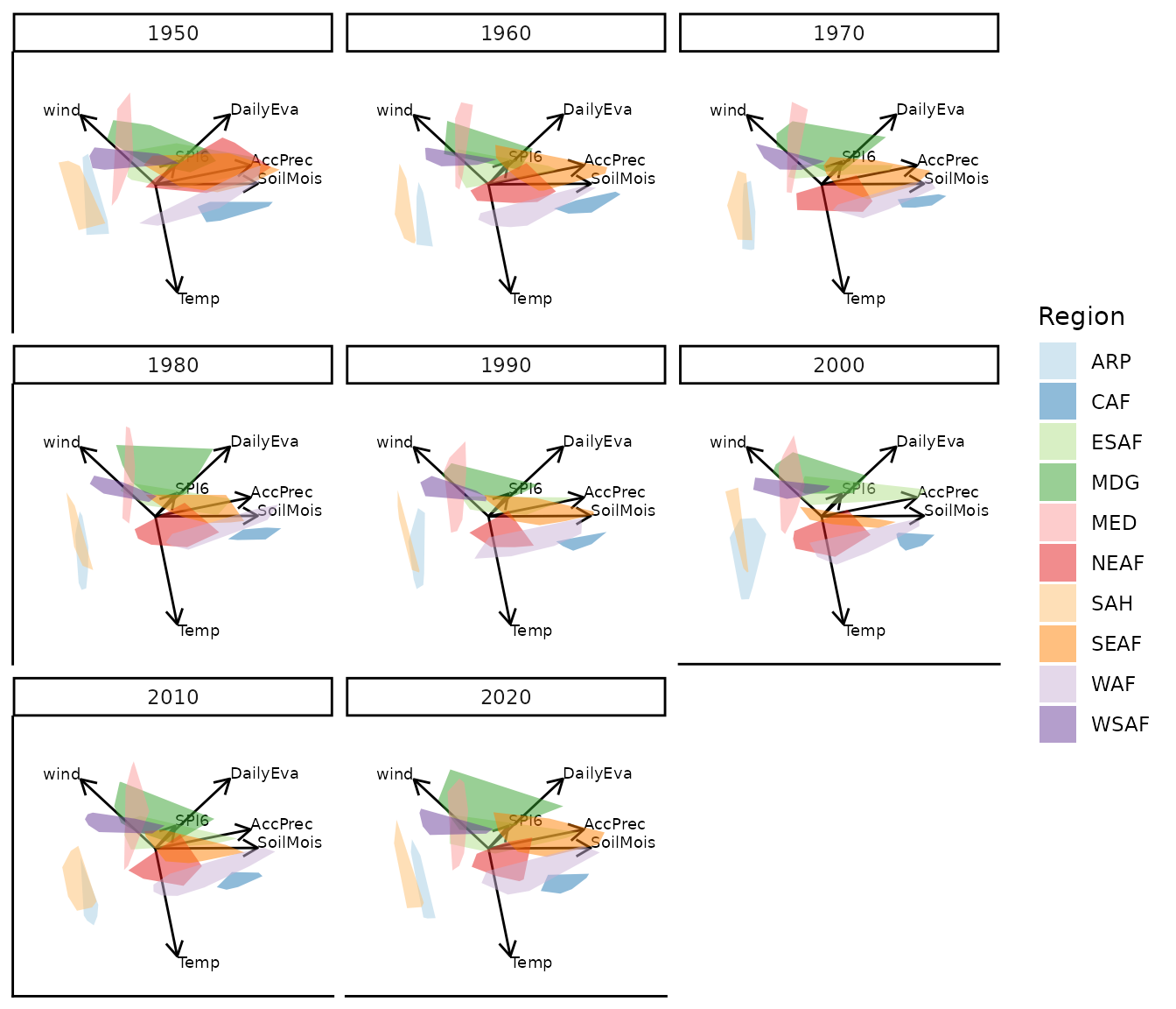

#> Object of class biplot, based on 960 samples and 9 variables.
#> 6 numeric variables.
#> 3 categorical variables.

Custom plotting characters and opacity

bp_pch <- biplotEZ::biplot(Africa_climate, scaled = TRUE,
                            group.aes = Africa_climate$Region) |>
  biplotEZ::PCA() |>
  biplotEZ::samples(pch = c(22, 21, 24, 23), opacity = 0.4)

bp_pch |> moveplot(time.var = "Year", group.var = "Region",
                   hulls = FALSE, move = FALSE)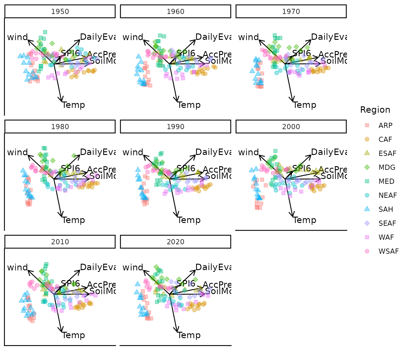

#> Object of class biplot, based on 960 samples and 9 variables.
#> 6 numeric variables.
#> 3 categorical variables.

Note that pch values cycle across the ten region groups — specify ten values to assign a unique character to each region.

References

Gower, J. C., and G. B. Dijksterhuis. 2004. Procrustes Problems. Book. Oxford University Press.

Hersbach, Hans, Bill Bell, Paul Berrisford, et al. 2023. ERA5 hourly data on single levels from 1940 to present. Copernicus Climate Change Service (C3S) Climate Data Store (CDS). https://doi.org/10.24381/cds.adbb2d47.

Iturbide, M., J. M. Gutiérrez, L. M. Alves, et al. 2020. “An Update of IPCC Climate Reference Regions for Subcontinental Analysis of Climate Model Data: Definition and Aggregated Datasets.” Earth System Science Data 12 (4): 2959–70. https://doi.org/10.5194/essd-12-2959-2020.

Lubbe, Sugnet, Niël le Roux, Johané Nienkemper-Swanepoel, et al. 2024. biplotEZ: EZ-to-Use Biplots. https://doi.org/10.32614/CRAN.package.biplotEZ.

Nienkemper-Swanepoel, J., N. J. le Roux, and S. Gardner-Lubbe. 2023. “GPAbin: Unifying Visualizations of Multiple Imputations for Missing Values.” Communications in Statistics - Simulation and Computation 52 (6): 2666–85. https://doi.org/10.1080/03610918.2021.1914089.

Overview

Data

Fixed Variable Frame: moveplot()

Static faceted display

Animated display

Dynamic Frame: moveplot2()

Static faceted display (unaligned)

Static faceted display (aligned)

Animated display

Automated Alignment: moveplot3()

Consensus target (target = NULL)

Static faceted display

Animated display

User-supplied target (target = Africa_climate_target)

Static faceted display

Animated display

Evaluation

Numerical measures

Fit measures over time

Bias measures over time

Additional Examples

Alternative use of time.var

Customising aesthetics

Custom colour palette and axis label size

Custom plotting characters and opacity

References

Fixed Variable Frame: `moveplot()`

Dynamic Frame: `moveplot2()`

Automated Alignment: `moveplot3()`

Consensus target (`target = NULL`)

User-supplied target (`target = Africa_climate_target`)

Alternative use of `time.var`