Correspondence Analysis (CA) method
CA.RdThis function produces a list of elements to be used for CA biplot construction by approximation of the Pearson residuals.
Arguments
- bp
object of class
biplotobtained from preceding functionbiplot(center = FALSE). In order to maintain the frequency table, the input should not be centered or scaled. ForCA,bpshould be a contingency table.- dim.biplot
dimension of the biplot. Only values 1, 2 and 3 are accepted, with default
2.- e.vects
which eigenvectors (canonical variates) to extract, with default
1:dim.biplot.- variant
which correspondence analysis variant, with default "Princ", presents a biplot with rows in principal coordinates and columns in standard coordinates.
variant = "Stand", presents a biplot with rows in standard coordinates and columns in principal coordinates.variant = "symmetric", presents a symmetric biplot with row and column standard coordinates scaled equally by the singular values.- lambda.scal
logical value to request lambda-scaling, default is
FALSE. Controls stretching or shrinking of column and row distances.
Value
A list with the following components is available:
- Z
Combined data frame of the row and column coordinates.
- r
Numer of levels in the row factor.
- c
Numer of levels in the column factor.
- Dr
Diagonal matrix of row profiles.
- Dc
Diagonal matrix of column profiles.
- Drh
Weighted row profiles.
- Dch
Weighted column profiles.
- rowcoor
Row coordinates based on the selected
variant.- colcoor
Column coordinates based on the selected
variant.- P
Correspondence Matrix.
- Smat
Standardised Pearson residuals.
- SVD
Singular value decomposition solution:
d, u, v.- e.vects
Depending on what was specified in
CAargument.- dim.biplot
The dimension of the biplot.
- lambda.val
The computed lambda value if lambda-scaling is requested.
- gamma
Contribution of the singular values, based on the CA variant.
Examples
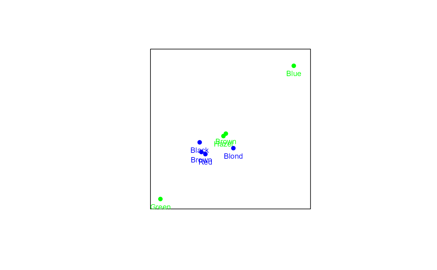
# Creating a CA biplot with rows in principal coordinates:
biplot(HairEyeColor[,,2], center = FALSE) |> CA() |> plot()
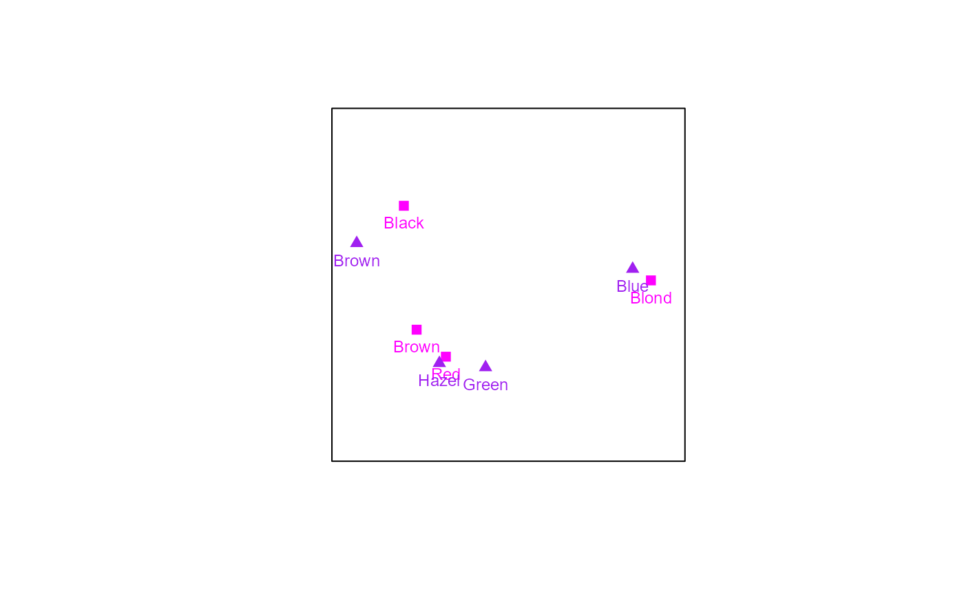
 # Creating a CA biplot with rows in standard coordinates:
biplot(HairEyeColor[,,2], center = FALSE) |> CA(variant = "Stand") |>
samples(col=c("magenta","purple"), pch = c(15,17), label.col = "black") |> plot()
# Creating a CA biplot with rows in standard coordinates:
biplot(HairEyeColor[,,2], center = FALSE) |> CA(variant = "Stand") |>
samples(col=c("magenta","purple"), pch = c(15,17), label.col = "black") |> plot()
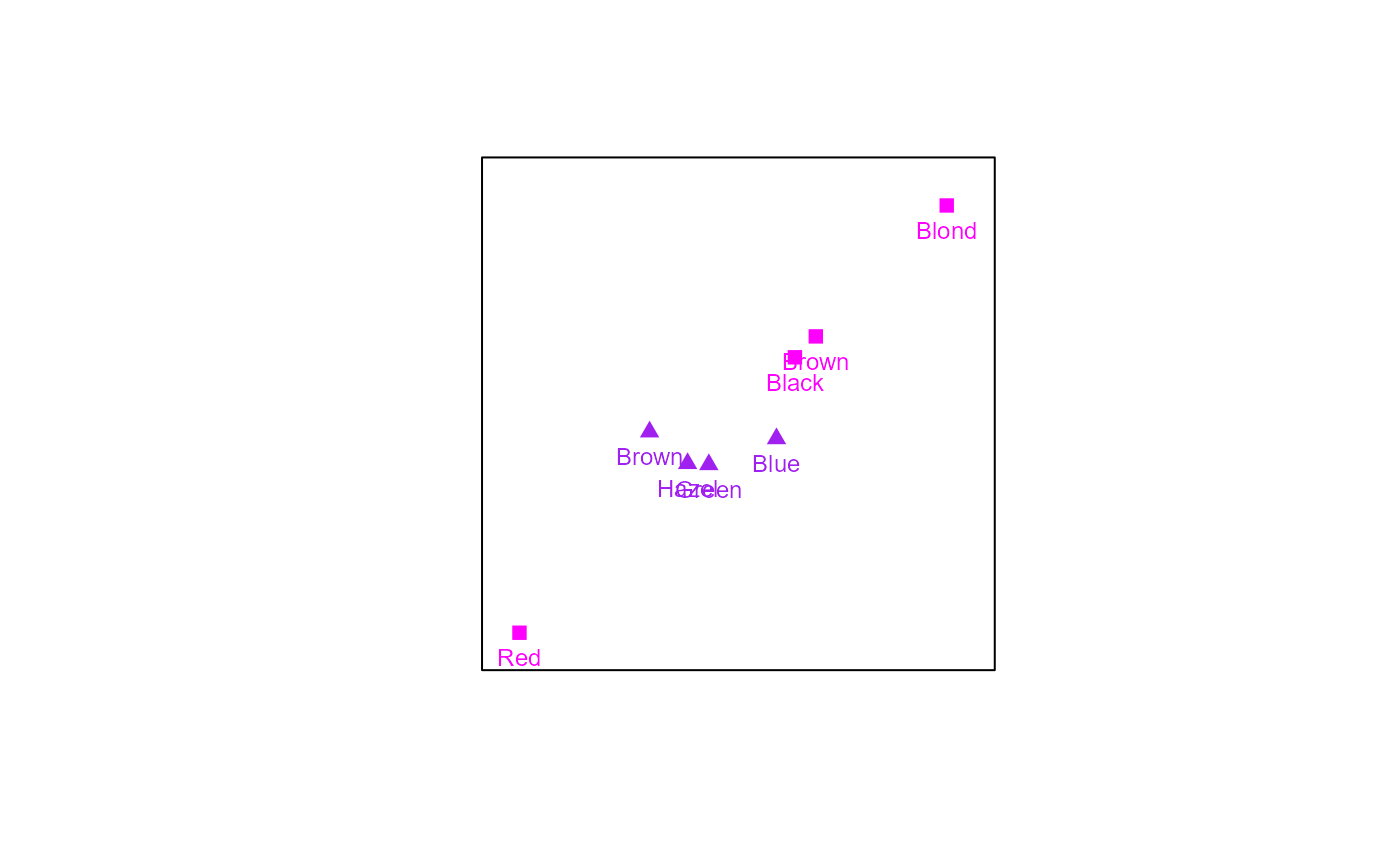 # Creating a CA biplot with rows and columns scaled equally:
biplot(HairEyeColor[,,2], center = FALSE) |> CA(variant = "Symmetric") |>
samples(col = c("magenta","purple"), pch = c(15,17), label.col = "black") |> plot()
# Creating a CA biplot with rows and columns scaled equally:
biplot(HairEyeColor[,,2], center = FALSE) |> CA(variant = "Symmetric") |>
samples(col = c("magenta","purple"), pch = c(15,17), label.col = "black") |> plot()