First step to create a new biplot with biplotEZ

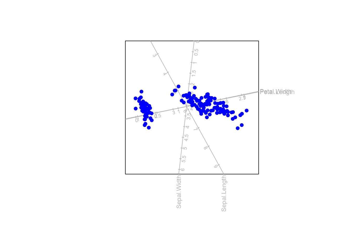
This function produces a list of elements to be used when producing a biplot, which provides a useful data analysis tool and allows the visual appraisal of the structure of large data matrices. Biplots are the multivariate analogue of scatter plots. They approximate the multivariate distribution of a sample in a few dimensions and they superimpose on this display representations of the variables on which the samples are measured.

biplot(data, classes = NULL, group.aes = NULL, center = TRUE, scaled = FALSE,
Title = NULL)

Arguments

data: a data frame or numeric matrix containing all variables the user wants to analyse.
classes: a vector identifying class membership.
group.aes: a vector identifying groups for aesthetic formatting.
center: a logical value indicating whether data should be column centered, with default TRUE.
scaled: a logical value indicating whether data should be standardised to unit column variances, with default FALSE.
Title: the title of the biplot to be rendered, enter text in " ".

Value

A list with the following components is available:

X: the matrix of the centered and scaled numeric variables.
Xcat: the data frame of the categorical variables.
raw.X: the original data.
classes: the vector of category levels for the class variable. This is to be used for colour, pch and cex specifications.
na.action: the vector of observations that have been removed.
center: a logical value indicating whether \(\mathbf{X}\) is centered.
scaled: a logical value indicating whether \(\mathbf{X}\) is scaled.
means: the vector of means for each numeric variable.
sd: the vector of standard deviations for each numeric variable.
n: the number of observations.
p: the number of variables.
group.aes: the vector of category levels for the grouping variable. This is to be used for colour, pch and cex specifications.
g.names: the descriptive names to be used for group labels.
g: the number of groups.
Title: the title of the biplot rendered

Details

This function is the entry-level function in biplotEZ to construct a biplot display. It initialises an object of class biplot which can then be piped to various other functions to build up the biplot display.

Useful links

The biplot display can be built up in four broad steps depending on the needs for the display. Firstly, choose an appropriate method to construct the display; Secondly, change the aesthetics of the display; Thirdly, append the display with supplementary features such as axes, samples and means; Finally, superimpose shapes, characters or elements onto the display.

1. Different types of biplots:

PCA(): Principal Component Analysis biplot of various dimensions
CVA(): Canonical Variate Analysis biplot
PCO(): Principal Coordinate Analysis biplot
CA(): Correspondence Analysis biplot
regress(): Regression biplot method

2. Customise the biplot display with aesthetic functions:

samples(): Change the formatting of sample points on the biplot display
axes(): Change the formatting of the biplot axes

3. Supplement the existing biplot with additional axes, samples and group means:

newsamples(): Add and change formatting of additional samples
newaxes(): Add and change formatting of additional axes
means(): Insert class means to the display, and format appropriately

4. Append the biplot display:

alpha.bags(): Add \(\alpha\)-bags
ellipses(): Add ellipses
density2D(): Add 2D density regions

Other useful links:

References

Gabriel, K.R. (1971) The biplot graphic display of matrices with application to principal component analysis. Biometrika. 58(3):453–467.

Gower, J., Gardner-Lubbe, S. & Le Roux, N. (2011, ISBN: 978-0-470-01255-0) Understanding Biplots. Chichester, England: John Wiley & Sons Ltd.

Gower, J.C. & Hand, D.J.(1996, ISBN: 0-412-71630-5) Biplots. London: Chapman & Hall.

Examples

biplot(data = iris)
#> Object of class biplot, based on 150 samples and 5 variables.
#> 4 numeric variables.
#> 1 categorical variable.
# create a PCA biplot
biplot(data = iris) |> PCA() |> plot()